Multivariable Calculus 27 | Application of the Implicit Function Theorem

TL;DR

The implicit function theorem can be upgraded to preserve differentiability class: C^k (including C^∞) input yields a C^k (including C^∞) implicit function when the Jacobian is invertible.

Briefing Cornell Notes

Briefing

A simple zero of a polynomial doesn’t just exist—it moves smoothly when the polynomial’s coefficients are perturbed. That stability is the payoff of the implicit function theorem in a multivariable setting, and it replaces the “closed-form” comfort of the quadratic formula with a general, differentiability-based guarantee.

The discussion starts by laying out the generalized inverse function theorem and then using it to justify a higher-regularity version of the implicit function theorem. If a function is continuously differentiable (or more generally C^k, including C^∞), and the relevant Jacobian determinant is invertible at a point, then the locally defined inverse/implicit function inherits the same differentiability class. In practice, this means that once the hypotheses are met, the implicit function not only exists locally but also depends smoothly on the parameters.

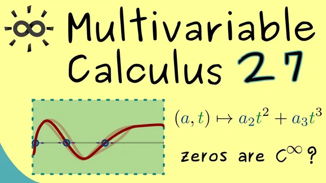
The application focuses on a real-coefficient polynomial P(t) with degree n and coefficients a0, a1, …, an. A “simple zero” t0 is defined by two conditions: P(t0)=0 and P′(t0)≠0. Geometrically, that nonzero derivative ensures the graph crosses the t-axis rather than merely touching it, and it’s exactly the condition that prevents the zero from becoming “degenerate” under perturbations.

To build the implicit function framework, the transcript first revisits the quadratic case as intuition: for a quadratic with A2≠0, the zeros can be written explicitly, and small coefficient changes lead to smoothly varying roots (at least locally, when the root remains simple). But for higher-degree polynomials, no general formula exists, so the implicit function theorem becomes the tool that guarantees smooth dependence without solving the polynomial.

For the general polynomial, a multivariable function F is constructed so that the polynomial equation becomes an implicit relation. The coefficients are treated as variables (renamed as x1, x2, …), while t plays the role of the remaining variable. The point x0 is chosen to encode the original coefficients together with the simple root t0. The key check is that the partial derivative of F with respect to the t-variable at that point is nonzero—equivalently, the 1×1 “Jacobian” (just the derivative) is invertible. With that condition satisfied, the implicit function theorem produces a local function G that returns the simple zero as a function of the coefficients.

The conclusion is practical: near a polynomial with a simple zero, small C^∞ changes in the coefficients produce a nearby simple zero that varies in a C^∞ way. The method fails precisely when the zero is not simple (when P′(t0)=0), because the invertibility condition breaks and smooth dependence can no longer be guaranteed. The transcript closes by pointing toward later topics—such as Lagrange multipliers—where these ideas reappear in a broader optimization context.

Cornell Notes

A polynomial’s simple zero is stable under small coefficient changes: if P(t0)=0 and P′(t0)≠0, then the root near t0 can be written locally as a smooth function of the coefficients. This stability comes from the implicit function theorem, which requires an invertible Jacobian (here, the partial derivative with respect to t at the root). The transcript also generalizes the inverse/implicit function theorems to C^k and C^∞ settings, ensuring that if the original function is smooth, the implicit function inherits the same smoothness. For quadratics, the quadratic formula already shows smooth dependence; for higher degrees, the implicit function theorem provides the same conclusion without needing an explicit root formula.

What exactly makes a zero “simple,” and why does that matter for stability?

A simple zero t0 satisfies two conditions: P(t0)=0 and P′(t0)≠0. The nonzero derivative means the graph crosses the t-axis rather than just touching it. In the implicit-function setup, this becomes the invertibility condition: the partial derivative of the constructed function F with respect to the t-variable at (coefficients, t0) is nonzero. That invertibility is what guarantees a locally unique root that changes smoothly when coefficients vary.

How does the implicit function theorem turn “solve P(t)=0” into “compute t as a function of coefficients”?

Instead of treating t as the only unknown, coefficients are treated as variables too. A multivariable function F is built so that F(coefficients, t)=0 is equivalent to P(t)=0. Then the implicit function theorem produces a local function G such that t = G(coefficients) and F(coefficients, G(coefficients))=0. In this construction, the coefficients are renamed as variables (x1, x2, …), and the chosen point x0 encodes the original coefficients together with the root t0.

Why is the Jacobian condition easy here, and what does it reduce to?

Because there is only one equation and one “t” variable, the Jacobian is effectively 1×1. The relevant derivative is ∂F/∂t at the point corresponding to the original coefficients and t0. That derivative equals the derivative of the polynomial at t0, so the condition becomes P′(t0)≠0. When this holds, the implicit function theorem applies directly.

Why does the transcript emphasize C^k and C^∞ versions of the theorems?

The smoothness of the implicit function G depends on the smoothness of F. Since polynomials are C^∞ in both t and the coefficients, F is C^∞. The generalized inverse/implicit function theorem then guarantees that G is also C^∞. So the root not only exists locally but also depends differentiably (indeed smoothly) on the coefficients.

What goes wrong when the zero is not simple?

If P′(t0)=0, the invertibility condition fails: the partial derivative ∂F/∂t at the corresponding point is zero. Without that, the implicit function theorem cannot guarantee a locally defined smooth function G for the root. In such cases, the root can split, merge, or behave non-smoothly under perturbations.

Review Questions

Given P(t0)=0 and P′(t0)≠0, what invertibility condition must hold in the implicit-function setup?
How does treating coefficients as variables change the problem compared with solving P(t)=0 directly?
Why does the quadratic formula illustrate the same phenomenon that the implicit function theorem guarantees for general polynomials?

Key Points

1
The implicit function theorem can be upgraded to preserve differentiability class: C^k (including C^∞) input yields a C^k (including C^∞) implicit function when the Jacobian is invertible.
2
A simple zero t0 of a polynomial satisfies P(t0)=0 and P′(t0)≠0, ensuring the root crosses the axis and enabling Jacobian invertibility.
3
By treating coefficients as variables, the polynomial equation P(t)=0 becomes an implicit relation F(coefficients, t)=0.
4
When ∂F/∂t is nonzero at the point corresponding to (original coefficients, t0), the implicit function theorem produces a local function t=G(coefficients).
5
Near a polynomial with a simple zero, small C^∞ perturbations of coefficients produce a nearby root that varies C^∞-smoothly.
6
If the zero is not simple (P′(t0)=0), the key invertibility condition fails, so smooth dependence of the root is not guaranteed.

Highlights

A simple root is stable: if P(t0)=0 and P′(t0)≠0, then the root persists locally and depends smoothly on coefficients.

The Jacobian condition collapses to a single derivative check: ∂F/∂t ≠ 0, which is exactly P′(t0)≠0.

For higher-degree polynomials, the implicit function theorem replaces explicit root formulas by guaranteeing smooth local dependence.

Smoothness transfers: because polynomials are C^∞, the implicit root function G is also C^∞ near a simple zero.

Topics

Implicit Function Theorem
Inverse Function Theorem
Simple Zeros
Stability Under Perturbations
C^Infinity Regularity