Regression Analysis: Assumptions, Interpretation, and Reporting in #SPSS with AI
Based on Research With Fawad's video on YouTube. If you like this content, support the original creators by watching, liking and subscribing to their content.
Check normality using skewness and kurtosis in SPSS Descriptives, treating values within ±2 as acceptable.
Briefing
Regression analysis in SPSS hinges on two things: checking core statistical assumptions before trusting the model, then reporting results in a way that ties hypothesis tests to the output tables. This workflow uses life satisfaction as a continuous dependent variable and ethical behavior (BE) and self-efficacy (SE) as predictors, with SPSS diagnostics used to confirm normality, linearity, independence of errors, multicollinearity, and homoscedasticity.
First, the dependent variable’s distribution is assessed using skewness and kurtosis from SPSS Descriptives. Skewness and kurtosis values fall within ±2, which is treated as evidence that normality is not violated. Outliers are then checked with box plots via Explore: significant outliers would appear with an asterisk, but none are flagged, so the dataset is kept intact. Next comes linearity, evaluated through scatterplots of LS against BE and LS against SE; the points show a generally linear pattern with some scatter. AI-assisted interpretation is used to confirm the presence of positive linear relationships for both predictor pairs.
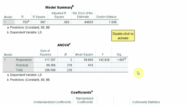
The independence and error-shape assumptions are handled through the regression diagnostics panel. Autocorrelation is checked with the Durbin–Watson statistic, reported as 1.63. Because Durbin–Watson ranges from 0 to 4 and values near 2 indicate no significant autocorrelation, 1.63 is treated as acceptable. Multicollinearity is assessed using collinearity diagnostics, specifically VIF values, which are reported as below 5 (and therefore not problematic). Residual normality is evaluated using a normal P–P plot of standardized residuals, where points lie close to the reference line. Finally, homoscedasticity is examined through the residuals-vs-predicted plot; a pattern is noted but judged not strong enough to seriously violate equal variance.
With assumptions cleared, the regression results are interpreted and prepared for reporting. The model tests whether ethical behavior and self-efficacy significantly predict life satisfaction. The overall model is significant: F(2, 28) = 142.929 with p < .001. The model explains 56.7% of variance in life satisfaction (R² = .567), meaning BE and SE account for roughly 56.7% of the variability in LS.
Individual coefficients then address the hypotheses. Ethical behavior (BE) shows a significant positive effect on life satisfaction with β = .454, t = 7.916, and p < .001, supporting H1. Self-efficacy (SE) also has a significant positive effect with β = .290, t = 4.950, and p < .001, supporting H2. The reporting guidance emphasizes including assumption checks (skewness/kurtosis, outliers, linearity, Durbin–Watson, VIF, residual normality, homoscedasticity) and then presenting the model summary (F, p, R²) followed by the coefficients table (β, t, p) in a research-paper-ready format.
Cornell Notes
The regression workflow in SPSS starts by validating assumptions before interpreting predictors. Life satisfaction (LS) is treated as continuous, with skewness and kurtosis within ±2 indicating no normality violation. Outliers are screened using box plots (significant outliers would be marked with an asterisk), and none are flagged. Linearity is checked via scatterplots of LS with ethical behavior (BE) and self-efficacy (SE), showing positive linear patterns. Independence of errors is evaluated with Durbin–Watson (1.63, close to 2), multicollinearity is checked with VIF (<5), residuals are assessed as approximately normal using a P–P plot, and homoscedasticity is judged acceptable from residual plots.
After diagnostics, the model predicts LS significantly: F(2, 28) = 142.929, p < .001, with R² = .567. Both predictors are significant and positive: BE (β = .454, t = 7.916, p < .001) and SE (β = .290, t = 4.950, p < .001).
Why are skewness and kurtosis checked before running regression, and what threshold is used here?
How does the outlier check work in SPSS, and what does an asterisk mean?
What does “linearity” mean here, and how is it assessed for both predictors?
Which diagnostics are used for independence and multicollinearity, and what are the decision rules?
How are residual normality and homoscedasticity evaluated?
How are the final regression results translated into hypothesis statements?
Review Questions
- What specific assumption checks are performed before interpreting regression coefficients, and what outputs in SPSS correspond to each assumption?
- How do Durbin–Watson and VIF function as decision tools for independence and multicollinearity, respectively?
- Given F(2, 28) = 142.929, p < .001 and R² = .567, what additional information from the coefficients table is needed to support H1 and H2?
Key Points
- 1
Check normality using skewness and kurtosis in SPSS Descriptives, treating values within ±2 as acceptable.
- 2
Screen outliers with box plots in SPSS Explore; significant outliers are labeled with an asterisk.
- 3
Verify linearity using scatterplots of LS against each predictor (BE and SE) and confirm the relationship is approximately linear.
- 4
Assess autocorrelation with Durbin–Watson; values close to 2 indicate no serious autocorrelation (here, 1.63).
- 5
Evaluate multicollinearity with VIF from collinearity diagnostics; VIF below 5 indicates no collinearity concern.
- 6
Confirm residual normality with a normal P–P plot of standardized residuals and check homoscedasticity using residual plots for equal variance.
- 7
Report results in a structured order: assumptions (briefly), overall model (F, df, p, R²), then coefficients (β, t, p) for each hypothesis.