The Insane Math Of Knot Theory
Based on Veritasium's video on YouTube. If you like this content, support the original creators by watching, liking and subscribing to their content.
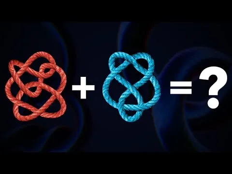
Knot theory models knots as closed loops and defines equivalence as transformability without breaking the loop.
Briefing
Knot theory turns “tangled rope” into a rigorous system for distinguishing shapes that can’t be untied without cutting—an effort that now underpins everything from DNA replication to new materials. The central challenge is the knot equivalence problem: deciding whether two knots are the same up to continuous deformation. That question resisted systematic answers for more than a century, even as researchers built massive catalogs of knots and developed powerful mathematical “fingerprints” to tell them apart.
In knot theory, knots live on closed loops, so the simplest knot is the unknot (a plain circle). Two knots are considered different if one can’t be transformed into the other without breaking the loop. Visually, even simple knots can be hard to tell apart, and the transcript highlights how a “mystery knot” can be a trefoil—or how an apparently complex tangle can actually be just an unknot once it’s disentangled.
The equivalence problem became famous through historical attempts to classify knots like a periodic table. In the late 1800s, Scottish physicist Peter Guthrie Tait—after being inspired by Lord Kelvin’s vortex-ring model of atoms—tabulated knots by counting crossings in their simplest form. He and later collaborators Thomas Kirkman and Charles Little extended these lists up to seven crossings by hand, then continued up to ten crossings by 1899. Their work stood for decades, until a single correction in 1973 reduced the count of ten-crossing prime knots from 166 to 165 after Kenneth Perko identified a “Perko pair” that had been mistakenly treated as distinct.
A breakthrough came in 1927 when Kurt Reidemeister proved that knot equivalence can be checked using only three local moves—twist, poke, and slide. If two knots can be connected by a sequence of these moves, they’re the same. But proving two knots are different is far harder: Reidemeister moves can be applied indefinitely without revealing a mismatch.
Computational progress eventually made the problem decidable in practice for broad classes. In 1961, Wolfgang Haken produced an algorithm to distinguish any knot from the unknot, though it was computationally infeasible for large cases. Later work tightened bounds on how many Reidemeister moves must be checked, shrinking the worst-case search from astronomically large numbers to still-unimaginable ones. By 2011, researchers established an upper bound that—at least in principle—solves the entire knot equivalence problem, even though the resulting numbers grow via tetration and remain beyond brute-force computation.
To manage the scale of classification, knot theorists rely on invariants—quantities unchanged under Reidemeister moves. Crossing number is one invariant but is difficult to compute reliably. More practical are coloring invariants like tricolorability and its generalization, p-colorability, which can prove that the trefoil is not the unknot. Polynomial invariants provide even sharper tools: the Alexander polynomial, then the Jones polynomial (discovered by Vaughan Jones after work resembling statistical mechanics equations), and later the HOMFLY and HOMFLY-PT polynomials. No single invariant is perfect, so researchers combine many to uniquely identify knots.
That mathematical machinery now feeds real-world applications. Synthetic chemists have tied molecular knots, starting with Jean-Pierre Sauvage’s trefoil around copper ions, and later creating an 819-knot record bound to a chloride ion. In biology, type two topoisomerase enzymes cut and rejoin DNA to reduce knotting during replication; inhibiting these enzymes underlies the action of quinolone antibiotics and many chemotherapy strategies. Even everyday shoelace behavior maps onto knot types: the “granny knot” and “square knot” differ by mirror-image trefoils, with the clockwise version typically less prone to loosening. The result is a field that began as a curiosity about rope loops and evolved into a toolkit for materials, medicine, and molecular design—while still wrestling with the deep logic of when two knots truly match.
Cornell Notes
Knot theory studies closed-loop tangles and asks whether two knots are equivalent without cutting. The knot equivalence problem—deciding if two knots can be transformed into each other—was historically difficult, but Reidemeister’s three local moves (twist, poke, slide) provide the framework for proving equivalence. Proving inequivalence is harder, so mathematicians use invariants such as crossing number, coloring tests (tricolorability and p-colorability), and polynomial invariants like the Alexander polynomial and the Jones polynomial. These tools enabled massive knot tabulations, including a corrected count of prime knots up to 10 crossings and later computational expansions to hundreds of millions. The payoff extends beyond math: knot structure matters in DNA replication, antibiotic and chemotherapy mechanisms, and the design of synthetic knotted molecules.
What makes two knots “the same” in knot theory, and why does that definition matter for classification?
How did Reidemeister’s theorem change the knot equivalence problem?
Why are invariants essential when equivalence proofs are difficult?
What was the significance of the “Perko pair” correction to Tait’s knot tables?
How do knot invariants connect to real-world chemistry and biology?
How does the shoelace example map onto knot theory concepts?
Review Questions
- What does Reidemeister’s theorem guarantee, and what does it fail to guarantee about proving two knots are different?
- Give one example of an invariant (coloring or polynomial) and describe how it can prove the unknot is not the trefoil.
- Why did the number of prime knots up to 10 crossings change after the Perko correction, and what does that reveal about relying on early classification methods?
Key Points
- 1
Knot theory models knots as closed loops and defines equivalence as transformability without breaking the loop.
- 2
Reidemeister’s three local moves (twist, poke, slide) provide a complete method for proving two knots are the same.
- 3
Proving two knots are different relies heavily on invariants, since inequivalence can be hard to certify directly.
- 4
Coloring invariants (tricolorability and p-colorability) can distinguish the trefoil from the unknot, even when visual inspection fails.
- 5
Polynomial invariants—Alexander, Jones, HOMFLY, and HOMFLY-PT—offer stronger discrimination, but no single invariant is sufficient on its own.
- 6
Massive knot tabulations grew from hand counting (Tait, Kirkman, Little) to computer-assisted enumeration, reaching 352,152,252 known prime knots.
- 7
Knot structure is not just abstract: it influences DNA replication via type two topoisomerases, antibiotic/chemotherapy mechanisms, and the design of synthetic knotted molecules.