What Textbooks Don't Tell You About Curve Fitting
Based on Artem Kirsanov's video on YouTube. If you like this content, support the original creators by watching, liking and subscribing to their content.
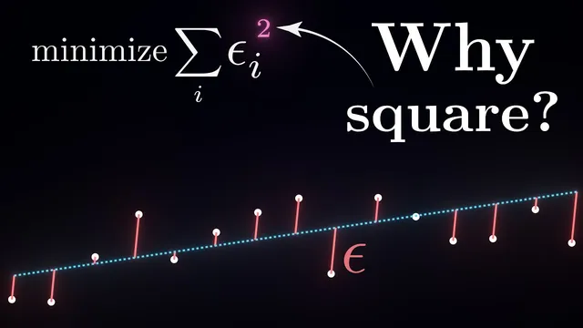
Least squares arises as the maximum-likelihood solution for a linear model with additive Gaussian noise, making the squared residual term a consequence of the noise assumption.
Briefing
Linear regression’s familiar “minimize squared vertical errors” rule isn’t just a convenient math trick—it drops out of a probabilistic assumption about noise. By treating observed outputs as a linear function of inputs plus random error, then choosing the parameters that make the observed data most likely, the optimization objective becomes least squares. The squared term appears because the noise is assumed to be Gaussian: under that assumption, maximizing the probability of the data is equivalent to minimizing the sum of squared differences between predicted and observed values.
That probabilistic framing also answers why “vertical distances” and “squares” show up in the first place. The model imagines a cloud of plausible outcomes around the predicted value for any given input, with the cloud’s shape determined by the noise distribution. When each data point is treated as an independent draw, the overall likelihood of the dataset is the product of per-point probabilities; taking logs turns that product into a sum, and the Gaussian form collapses neatly into the squared-error objective. In short: least squares is the maximum-likelihood solution for a linear model with additive Gaussian noise.
The discussion then pivots to what happens when multiple parameter settings fit the data equally well—or when “fit the data” conflicts with prior beliefs. A coin-bias example shows the limitation of pure maximum-likelihood: observing 4 heads out of 5 pushes the estimate toward 0.8, even though experience suggests most coins are near 0.5. The fix is to incorporate priors over parameters, selecting weights that jointly explain the data and align with expectations. Mathematically, this becomes maximizing the joint probability of data and parameters, which decomposes into a likelihood term (data fit) times a prior term (parameter plausibility).
From that joint-probability view, regularization stops being an arbitrary penalty and becomes a direct consequence of choosing a prior distribution over weights. Assuming weights follow a zero-centered Gaussian prior yields L2 regularization (ridge regression), which penalizes the squared magnitude of coefficients and gently shrinks them toward zero. The strength of the penalty is governed by the ratio between noise variance (how trustworthy the data are) and the prior variance (how strongly the prior expects weights to be small).
Assuming instead that weights are likely exactly zero except for a few important ones leads to a Laplace (double-exponential) prior, producing L1 regularization (lasso). Because L1 penalizes absolute values rather than squares, it more readily drives many coefficients to exactly zero, creating sparse models. The transcript links this sparsity preference to domains like genomics and neuroscience, where only a small subset of features or neurons typically matters for a given outcome.
Overall, the core takeaway is that least squares and common regularizers are not separate inventions: they are maximum-likelihood and maximum-a-posteriori solutions under specific noise and prior assumptions. Change those assumptions—Gaussian vs. non-Gaussian noise, or Gaussian vs. Laplace priors—and the resulting objectives change in predictable, principled ways. That same probabilistic logic extends beyond linear regression to much broader machine learning systems, where modeling assumptions often determine what “good behavior” looks like.
Cornell Notes
Linear regression’s least-squares objective emerges from maximum-likelihood estimation under a Gaussian noise model. Treat each observed target as a linear prediction plus additive error; assuming the error is normally distributed makes maximizing the probability of the data equivalent to minimizing the sum of squared prediction errors. When multiple parameter settings fit similarly—or when experience suggests parameters should behave a certain way—pure likelihood can be misleading, as illustrated by the biased-coin example. Incorporating prior beliefs leads to maximizing joint probability (likelihood × prior), which produces regularization. A Gaussian prior over weights yields L2 (ridge) regularization, while a Laplace prior yields L1 (lasso) regularization and encourages sparsity.
Why does least squares use squared vertical errors rather than absolute errors or other powers?
How does the probabilistic view turn “fit the data” into an optimization objective?
What goes wrong with maximum-likelihood regression when parameters are underconstrained?
How do priors over weights produce regularization?
Why does a Gaussian prior lead to L2 regularization (ridge)?
Why does a Laplace prior lead to L1 regularization (lasso) and sparsity?
Review Questions
- In what exact way does the Gaussian noise assumption mathematically force the residuals to be squared in the regression objective?
- How does maximizing P(data, w) differ from maximizing P(data|w), and how does that difference translate into regularization terms?
- What prior over weights would you choose if you believed most coefficients should be exactly zero, and why would that choice encourage sparsity?
Key Points
- 1
Least squares arises as the maximum-likelihood solution for a linear model with additive Gaussian noise, making the squared residual term a consequence of the noise assumption.
- 2
Assuming independent data points turns the dataset likelihood into a product of per-point probabilities; taking logs converts it into a sum that yields the standard quadratic objective.
- 3
Pure maximum-likelihood can produce implausible parameter values when data are limited, because it ignores prior expectations about what parameters should look like.
- 4
Regularization can be derived by maximizing joint probability (likelihood × prior), turning prior beliefs about weights into explicit penalty terms.
- 5
A zero-centered Gaussian prior over weights yields L2 regularization (ridge), which shrinks all coefficients toward zero without forcing exact zeros.
- 6
A Laplace prior over weights yields L1 regularization (lasso), which penalizes absolute values and more strongly encourages exact sparsity.
- 7
The regularization strength λ reflects the trade-off between noise variance (how much to trust the data) and prior variance (how strongly to trust prior beliefs about weights).