Differential Equations: The Language of Change

TL;DR

Neurons are modeled as dynamical systems whose present behavior depends on their evolving state over time, not just instantaneous input.

Briefing Cornell Notes

Briefing

Neurons behave less like simple input-output switches and more like time-dependent dynamical systems whose current response depends on their past. That temporal dependence is best understood through differential equations—the mathematical “language of change”—paired with geometric tools such as phase portraits and limit cycles, which reveal how complex behavior can emerge even from simple rules.

The foundation starts with dynamical systems theory: describe a system at any moment using state variables—real numbers that fully determine the system’s relevant state. For a ball in 3D space, position (x, y, z) and velocity components specify the state; for a pendulum, the angle and angular velocity suffice under simplifying assumptions. The choice of state variables is an abstraction decision: a neuron’s computational model focuses on electrical properties while ignoring other biochemical details, whereas a biochemist might do the reverse.

Differential equations then formalize how state variables change over time. Using a bacteria population in a Petri dish as an example, the growth rate is proportional to the current population: the rate of change dN/dt equals K·N, where K depends on conditions like temperature and food. The derivative is interpreted geometrically as the slope of the tangent to the population-vs-time curve. Real modeling, however, requires numerical methods rather than idealized infinitesimal changes: replace d with Δ and update the population in finite time steps. Measuring every five minutes instead of continuously assumes the rate stays roughly constant over that interval, enabling step-by-step predictions. This numerical approach matters because most differential equations—especially those relevant to neurons—lack closed-form solutions, so computation becomes the practical route.

Numerical solving also introduces tradeoffs and uncertainty. Smaller time steps improve accuracy but demand more computation. Parameter values like K are often unknown and must be inferred from data, meaning multiple simulations may be needed to fit observations, with finite precision inevitably leaving errors.

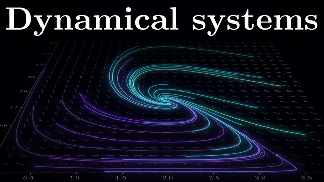
To build intuition for richer dynamics, the discussion shifts to coupled differential equations via a predator-prey model (rabbits and foxes). Rabbits grow proportionally to their population but decline when eaten by foxes, producing an interaction term −bxy. Foxes increase by converting consumed rabbits into reproduction (+cxy) but decline naturally without prey (−dy). Plotting time-series curves is useful, but the key geometric move is phase space: axes represent the two populations (x and y), while arrows at each point show the instantaneous direction of change. Equilibrium points occur where both derivatives vanish; one equilibrium is the trivial extinction state (0,0), while another represents a balance between predators and prey.

Around the extinction point, small perturbations drive the system away in one direction and toward extinction in another, signaling instability. Near the nonzero equilibrium, trajectories can form a closed loop—a limit cycle—meaning oscillations arise without explicitly inserting periodic functions. Changing assumptions can also transform behavior: limiting rabbit food can collapse the system from many possible cycles into a single stable equilibrium where trajectories converge.

These same geometric ideas—stability, equilibria, and limit cycles—are presented as the conceptual bridge to neuronal dynamics, where state variables may correspond to membrane potential and ion-channel states. The next step is promised as a dive into cellular biophysics to connect the math directly to how neurons generate spiking, bursting, and adaptation.

Cornell Notes

The core idea is that neurons can be treated as dynamical systems: their behavior at a moment depends on their state history, not just instantaneous input. Differential equations describe how state variables change over time, and numerical methods approximate derivatives using finite steps (Δ) because most realistic equations lack closed-form solutions. A bacteria-growth example turns the rule “growth rate is proportional to current population” into a differential equation and then into a step-by-step computation. To understand complex behavior without heavy calculation, the predator-prey model uses phase space, equilibrium points, and phase portraits; it can produce limit cycles—persistent oscillations emerging from interaction terms alone. These geometric concepts set up later applications to neuronal spiking and bursting.

What makes a dynamical system “fully described” at a given time, and how do state variables fit in?

A dynamical system is characterized by state variables—real numbers that, once known, determine everything relevant about the system’s current state. For a ball moving in 3D, the state can be given by position (x, y, z) and velocity components (how fast it moves in each direction). For a pendulum, two variables—angle from vertical and angular velocity—are enough only under the abstraction that treats the pendulum as a single point. The same idea applies to neurons: electrical properties can be chosen as state variables while other biochemical details (like sugar concentration or DNA repair) are ignored, depending on the modeling goal.

How does the bacteria example turn “growth” into a differential equation, and what does the derivative mean geometrically?

The bacteria population N(t) grows continuously, so the rate of change of N is proportional to N itself: dN/dt = K·N. Here K is a condition-dependent constant (e.g., temperature or food availability). The derivative dN/dt is interpreted as the slope of the tangent line to the N vs. time curve at that moment—like a “speedometer” for population growth. This connects calculus to modeling continuous change.

Why switch from d to Δ in numerical methods, and what does that change in practice?

Numerical modeling replaces infinitesimal changes with small but measurable time steps. Using Δ means updating the population using finite increments rather than assuming perfectly continuous evolution. In the example, instead of measuring hourly, the model updates every five minutes, assuming the growth rate doesn’t change much over that short interval (the curve looks locally straight when zoomed in). After estimating N at the next step, the growth rate is recalculated and the process repeats to project forward.

What is phase space, and how does it help reveal behavior without plotting time on the axes?

Phase space uses the system’s state variables as coordinates—e.g., rabbits x on one axis and foxes y on the other—so each point represents a possible system state at an instant. Time is not an axis; instead, trajectories show how the system moves through states over time. At each point, the model provides two instantaneous rates of change (dx/dt and dy/dt), which can be drawn as arrows. A collection of these arrows forms a phase portrait, letting observers infer qualitative behavior by following the flow.

How do equilibrium points and limit cycles arise in the predator-prey model?

Equilibrium points occur where both derivatives are zero, meaning the system has no built-in tendency to change. In the predator-prey model, one equilibrium is (0,0), where both populations are extinct; it’s mathematically valid but dynamically unstable. A nonzero equilibrium corresponds to a balance between predators and prey. Near that nonzero point, trajectories can loop into a closed orbit called a limit cycle, producing sustained oscillations even though no explicit periodic functions are inserted. The specific orbit reached depends on initial conditions.

What role do parameter changes play in the qualitative dynamics of the predator-prey system?

Changing parameters like a, b, c, and d can shift the location of the nonzero equilibrium and alter the shape and amplitude of limit-cycle oscillations. But additional modeling changes—such as limited food for rabbits—can qualitatively change the outcome: instead of many possible cycling behaviors, trajectories converge to a single stable equilibrium. That illustrates how small structural assumptions can transform long-term dynamics.

Review Questions

In the bacteria-growth model dN/dt = K·N, what does K represent, and how would changing the time step (e.g., from 5 minutes to 1 minute) affect numerical accuracy and computation cost?
In phase space for the predator-prey model, what conditions define an equilibrium point, and how can stability be inferred from the direction of arrows near that point?
Why can limit cycles appear without any explicit oscillatory functions in the equations, and what determines which limit cycle a system follows?

Key Points

1
Neurons are modeled as dynamical systems whose present behavior depends on their evolving state over time, not just instantaneous input.
2
State variables are the chosen real-number quantities that fully determine the system’s relevant state at a moment; what counts as “relevant” depends on the modeling abstraction.
3
Differential equations relate a quantity to its rate of change, with derivatives interpretable as tangent slopes on time-series graphs.
4
Numerical methods replace infinitesimal changes (d) with finite steps (Δ), enabling simulation when closed-form solutions are unavailable.
5
Smaller time steps improve accuracy but increase computational cost, and unknown parameters must often be fitted from data, introducing finite-precision uncertainty.
6
Phase portraits translate coupled differential equations into geometric flow in phase space, making stability and long-term behavior visible without exhaustive computation.
7
In the predator-prey model, equilibrium points and limit cycles emerge from interaction terms alone, and added constraints (like limited food) can switch the system from oscillations to convergence.

Highlights

Differential equations turn “change over time” into a precise relationship between a state variable and its rate of change, with derivatives matching the slope of tangents on graphs.

Numerical solutions use finite time steps (Δ) to approximate continuous dynamics, which is essential because most realistic equations—especially in neuroscience—don’t have simple analytic formulas.

Phase space replaces time on the axes: trajectories show how the system moves through possible states, while arrows encode instantaneous rates of change.

Limit cycles can arise without inserting periodicity by hand; they emerge from the coupled interaction structure of the model.

Stability can flip qualitatively when assumptions change—such as limiting rabbit food—shifting outcomes from sustained cycles to a single stable equilibrium.