Lecture 07: Foundation Models (FSDL 2022)
Based on The Full Stack's video on YouTube. If you like this content, support the original creators by watching, liking and subscribing to their content.
Fine-tuning lets teams reuse large pre-trained models by updating only a small portion of weights, making adaptation faster when labeled data is limited.
Briefing
Foundation models are driving a shift in AI from task-specific systems toward general-purpose models built by scaling architecture, data, and compute—then adapting them through fine-tuning, prompting, and retrieval. The central puzzle is why performance keeps rising even as training demands explode, but the lecture’s through-line is practical: the same core Transformer machinery, scaled and paired with better data and training objectives, powers breakthroughs across language, code, and vision.
The lecture starts with fine-tuning as the bridge from “old school” machine learning to today’s foundation models. Traditional approaches rely on training from scratch, but when data is scarce, models pre-trained on massive corpora can be reused by updating only a small portion of the network—often by adding a few layers or replacing the top layers while keeping most weights frozen. In NLP, the early bottleneck was representing words: one-hot vectors don’t scale and don’t encode semantic similarity. Word embeddings fix this by mapping vocabulary items into dense vector spaces where similarity reflects meaning, learned from co-occurrence patterns.
From there, the Transformer becomes the key architectural leap. “Attention is all you need” popularized an encoder-decoder design, but the lecture emphasizes the decoder-only setup used by GPT-style models. Self-attention turns each token into a weighted mixture of other tokens, with learned query/key/value projections and positional encoding to restore order. Layer normalization stabilizes training by keeping activations well-behaved across layers. Scaling then matters: modern models use dozens of layers and heads, large embedding dimensions, and huge parameter counts.
The lecture maps major model families and training regimes. GPT and GPT-2 are decoder-only language models trained to predict the next word, with performance improving as parameters grow. BERT flips the script with an encoder-only masked-word objective. T5 reframes tasks as text-to-text problems using both encoder and decoder components. GPT-3’s 175B parameters are highlighted for “emergent” few-shot and zero-shot behavior, and instruct-style tuning is credited for better instruction following via reinforcement learning with human rankings. Retrieval-augmented approaches like DeepMind’s RETRO aim to reduce reliance on memorized facts by fetching relevant text from large databases at inference time.
A major theme is scaling laws and data efficiency. Chinchilla results suggest many earlier models were “undertrained” for their parameter counts: better performance comes from using more tokens and fewer parameters under a fixed compute budget. That leads to a blunt takeaway—data sets deserve as much attention as model architectures, since optimal performance depends on both.
The lecture then shifts from language to applications. Prompt engineering is treated as an engineering layer over tokenization quirks: byte-pair encoding can break character-level tasks, while “scratch pad” style step-by-step prompting can improve multi-step reasoning. It also warns about prompt injection and “possessed” outputs in real systems.
For code, the lecture highlights filtering and verification as accuracy boosters: AlphaCode generates candidate solutions, then narrows them using models and execution. In general, separating generation from validation can lift results. It also describes tools like GitHub Copilot and research ideas like WebGPT, where models write code that is executed to answer questions.
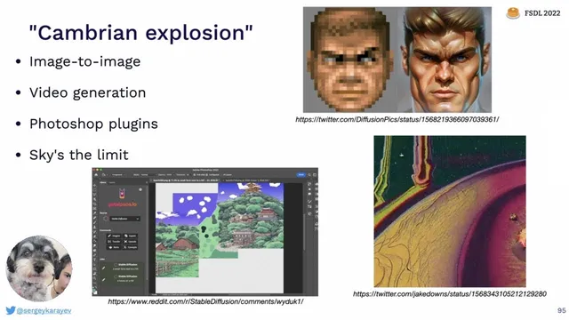
Finally, the lecture broadens to multimodal foundation models. CLIP aligns image and text embeddings using contrastive training, enabling zero-shot classification and cross-modal search. Image generation is explained through diffusion-based pipelines: models like DALL·E 2 use a diffusion prior to map text embeddings to image embeddings, then a decoder diffusion model to produce pixels. Stable Diffusion is presented as a latent diffusion alternative with open weights and a large public training dataset, fueling rapid community experimentation.
Overall, foundation models unify language, vision, and code under scalable Transformer-based systems, with performance increasingly driven by data quality, training objectives, retrieval, and post-generation verification—turning “prompting” and “fine-tuning” into the practical interfaces for real-world use.
Cornell Notes
Foundation models deliver broad capabilities by scaling Transformers with more data and compute, then adapting them via fine-tuning, prompting, and retrieval. The lecture traces how embeddings and self-attention enable language understanding, and how decoder-only Transformers power GPT-style next-token prediction. Scaling laws (especially Chinchilla) argue that many models were undertrained: optimal performance depends strongly on the amount of training data, not just parameter count. Instruction tuning (e.g., InstructGPT) improves how well models follow user requests, while retrieval-augmented methods (e.g., RETRO) reduce reliance on memorized facts. Across applications—code generation, semantic search, and image generation—accuracy often improves when generation is paired with filtering, verification, or diffusion-based conditioning.
Why did NLP move from one-hot word vectors to embeddings, and what problem do embeddings solve?
How does self-attention work in a Transformer, and what role do query, key, and value play?
What changes when moving from an encoder-only model like BERT to a decoder-only model like GPT?
What does Chinchilla’s scaling-law result imply about how to allocate compute between parameters and training tokens?
Why does prompt engineering sometimes work like a “hack,” and what tokenization issue is highlighted by the word-reversal example?
How do CLIP and diffusion-based models differ in what they generate or predict?
Review Questions
- What architectural components (attention, positional encoding, normalization) are necessary for a Transformer to handle sequence order and stable training?
- How do masked-language modeling (BERT) and next-token prediction (GPT) change what the model learns and how it’s used?
- According to the lecture’s Chinchilla discussion, what trade-off between parameters and training tokens tends to yield better performance under fixed compute?
Key Points
- 1
Fine-tuning lets teams reuse large pre-trained models by updating only a small portion of weights, making adaptation faster when labeled data is limited.
- 2
Embeddings replace one-hot word vectors with dense vectors that capture semantic similarity, often learned from word co-occurrence and trained to make related words close in embedding space.
- 3
Transformers rely on self-attention with query/key/value projections plus positional encoding and layer normalization; scaling these components drives much of modern performance.
- 4
Decoder-only GPT-style models use masked self-attention and next-token prediction, while BERT-style encoder-only models use random masking and token reconstruction.
- 5
Scaling laws (not just parameter count) matter: Chinchilla results emphasize that using more training tokens can outperform models that are “undertrained” for their size.
- 6
Instruction tuning (e.g., InstructGPT) improves instruction following by training on human-ranked outputs, while retrieval-augmented models (e.g., RETRO) fetch external text to reduce stale or memorized knowledge.
- 7
In multimodal systems, CLIP aligns image/text embeddings for retrieval and zero-shot tasks, while diffusion models generate pixels by denoising—often using a text-to-embedding prior plus an image decoder.