Linear Algebra 53 | Eigenvalues and Eigenvectors

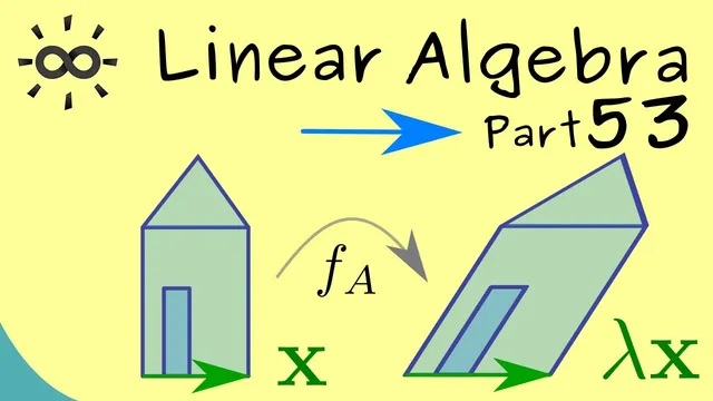
Eigenvalues and eigenvectors identify the special directions a linear transformation preserves—up to scaling—when a matrix acts on space. For a square matrix A representing a linear map f_A, an eigenvector x is any nonzero vector that, after applying the map, lands on the same line as before: f_A(x)=Ax=λx. The scalar λ is the eigenvalue, and it matters because it tells how that direction changes: λ>0 keeps the direction, λ<0 flips it, and λ=0 collapses the vector to the origin. This turns a geometric question about how a transformation reshapes space into an algebraic one about solving a matrix equation.

The core algebraic move is rewriting Ax=λx into (A−λI)x=0, where I is the identity matrix. That equation means x lies in the kernel (null space) of the matrix (A−λI). Since eigenvectors must be nonzero, the focus becomes finding values of λ for which (A−λI) has a nontrivial kernel. Once such an eigenvector exists, there are infinitely many eigenvectors for the same λ because any nonzero vector in that kernel can be scaled to produce another valid eigenvector. Geometrically, this is why eigenvectors correspond to “characteristic directions” of the transformation.

A worked 2×2 example illustrates the mechanics. Starting with a simple matrix (with entries chosen as 1s and 0s), the eigenvalue equation Ax=λx produces two component equations. The system is not linear in the unknowns because λ multiplies the vector components, so standard linear-system methods don’t apply directly. By analyzing the second equation first, one sees it is satisfied when λ=1 or when the relevant component x2=0. Checking each case against the first equation eliminates the options that lead only to the zero vector, leaving λ=1 as the only valid eigenvalue. Substituting λ=1 back into the equations forces x2=0 while leaving x1 free, yielding eigenvectors of the form (x1,0) with x1≠0. The example shows how eigenvalues can be determined by consistency conditions that prevent the solution from collapsing to the zero vector.

The formal definitions tie everything together. A scalar λ is an eigenvalue of A if there exists a nonzero vector x such that Ax=λx; that vector x is then an eigenvector. All eigenvectors associated with a fixed eigenvalue λ form an eigenspace, defined as the kernel of (A−λI). Unlike the set of eigenvectors themselves, the eigenspace is a subspace that includes the zero vector, which is included for convenience so the structure behaves like an ordinary subspace. Finally, the collection of all eigenvalues of A is called the spectrum of A. These definitions set up the systematic computation methods that come next.