Multivariable Calculus 29 | Method of Lagrange Multipliers

TL;DR

Constrained local extrema occur at points where the gradient of the objective is parallel to the gradient(s) defining the constraint(s).

Briefing Cornell Notes

Briefing

Lagrange multipliers for constrained extrema aren’t a special trick—they fall out directly from the implicit function theorem. For a function f(x1,x2) optimized along a constraint curve G(x1,x2)=0, a local extremum can only occur where the gradients of f and G point in the same direction (up to a scalar). That geometric condition matters because it turns a constrained optimization problem into a solvable system: instead of searching along a curve blindly, one checks where ∇f is parallel to ∇G.

The setup assumes two C1 functions: f is the objective, and G defines the constraint contour G=0. At a candidate point x̃, the constraint curve must be “nice enough,” meaning ∇G cannot vanish completely at that point. Under this nondegeneracy condition, the implicit function theorem rewrites the constraint locally as a graph: either x1=β(x2) or x2=γ(x1). Focusing on the case x2=γ(x1), the constraint becomes G(x1,γ(x1))=0 for x1 near the point. Because γ is C1, differentiating this identity with respect to x1 shows that ∇G(x̃) is orthogonal to the tangent direction of the constraint curve at x̃.

Next, the extremum condition is transferred from the original two-variable problem to a one-variable function along the constraint. Restricting f to the constraint curve yields a function of one variable, F̂(x1)=f(x1,γ(x1)). If x̃ is a local extremum of f subject to G=0, then F̂ has a local extremum at x1=x̃1, so its derivative must vanish. Applying the chain rule again gives that ∇f(x̃) is also orthogonal to the same tangent direction. In R2, any vector orthogonal to a fixed nonzero tangent direction must lie in a one-dimensional subspace, so ∇f(x̃) and ∇G(x̃) must both lie in that same line. Therefore there exists a real number λ such that ∇f(x̃)=λ∇G(x̃). This is exactly the Lagrange multiplier condition, derived from orthogonality plus the implicit function theorem rather than from ad hoc reasoning.

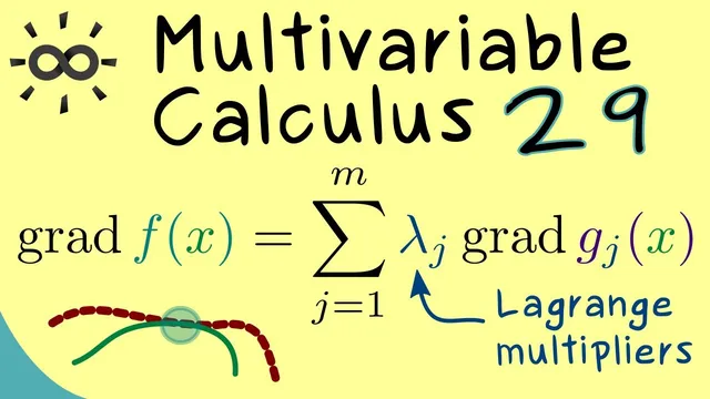
The same logic generalizes to higher dimensions. For f: R^n→R with constraints given by M functions G_j(x)=0 (j=1,…,M), the constraint set is described by a vector equation G(x)=0 in R^M. The implicit function theorem now requires a rank condition: the Jacobian of G at x̃ must have rank M, meaning the gradients ∇G_j span an M-dimensional subspace of R^n. At a constrained local extremum, ∇f(x̃) must lie in that span, so it can be written as a linear combination ∇f(x̃)=∑_{j=1}^M λ_j ∇G_j(x̃). The number of multipliers matches the number of independent constraints. The proof strategy remains the same—implicit function theorem for local parametrization, chain rule for differentiation, and an orthogonality/subspace argument at the end—while the detailed technicalities are deferred in favor of an example in the next segment.

Cornell Notes

Constrained extrema for f(x1,x2) with a constraint G(x1,x2)=0 occur only at points where ∇f is parallel to ∇G. The derivation uses the implicit function theorem to locally rewrite the constraint curve as a graph (e.g., x2=γ(x1)), then differentiates the identity G(x1,γ(x1))=0 to show ∇G is orthogonal to the constraint’s tangent direction. Restricting f to the constraint gives a one-variable function F̂(x1)=f(x1,γ(x1)); a local extremum forces F̂′(x̃1)=0, which via the chain rule makes ∇f orthogonal to the same tangent direction. In R2, that shared orthogonality pins both gradients to the same one-dimensional subspace, yielding ∇f(x̃)=λ∇G(x̃). The method extends to n variables and M constraints with a Jacobian rank condition, producing ∇f as a linear combination of ∇G_j.

Why does the implicit function theorem matter for Lagrange multipliers in two variables?

It guarantees the constraint curve G(x1,x2)=0 can be written locally as a graph near a candidate point x̃, provided ∇G(x̃) is not the zero vector. Concretely, one can locally express either x1=β(x2) or x2=γ(x1). That parametrization turns the constrained problem into an unconstrained one-variable problem along the curve, making differentiation possible with the chain rule.

How does differentiating G(x1,γ(x1))=0 lead to an orthogonality condition?

Once the constraint is written as x2=γ(x1), the identity G(x1,γ(x1))=0 holds for x1 in a neighborhood. Differentiating with respect to x1 gives ∇G(x̃)·(1,γ′(x̃1))=0. The vector (1,γ′(x̃1)) is tangent to the constraint curve at x̃, so ∇G(x̃) is orthogonal to the tangent direction.

Why does the extremum of f along the constraint force ∇f to be orthogonal to the same tangent direction?

Restricting f to the constraint yields a one-variable function F̂(x1)=f(x1,γ(x1)). If x̃ is a local extremum of f subject to G=0, then F̂ has a local extremum at x̃1, so F̂′(x̃1)=0. Applying the chain rule to F̂′(x̃1) produces ∇f(x̃)·(1,γ′(x̃1))=0. Thus ∇f(x̃) is orthogonal to the same tangent vector as ∇G(x̃).

What forces ∇f(x̃)=λ∇G(x̃) specifically in R2?

In R2, the orthogonal complement of a nonzero tangent direction is one-dimensional. Since both ∇f(x̃) and ∇G(x̃) are orthogonal to the same tangent vector, they must both lie in that same one-dimensional subspace. That means one gradient is a scalar multiple of the other: ∇f(x̃)=λ∇G(x̃).

How does the general M-constraint case change the condition on gradients?

With M constraints G_j(x)=0 in R^n, the Jacobian of G (whose rows are ∇G_j) must have rank M at x̃ to apply the implicit function theorem. Then the gradients ∇G_j span an M-dimensional subspace of R^n. The constrained extremum condition forces ∇f(x̃) to lie in that span, so ∇f(x̃)=∑_{j=1}^M λ_j ∇G_j(x̃).

What is the key rank condition and why is it needed?

The Jacobian of G must have rank M at x̃. This is the implicit function theorem’s requirement for local parametrization: it ensures the constraint set behaves like a smooth manifold of codimension M near x̃. Without full rank, the constraint might not be representable in the needed local form, and the gradient-subspace conclusion can fail.

Review Questions

For a constraint curve defined by G(x1,x2)=0, what nondegeneracy condition on ∇G at a candidate point is used to apply the implicit function theorem?
In the two-variable proof, which one-variable function is constructed from f and the constraint, and what condition on its derivative is used at the extremum?
In the n-variable, M-constraint generalization, what rank condition on the Jacobian of G is required, and what does it imply about the span of the gradients ∇G_j?

Key Points

1
Constrained local extrema occur at points where the gradient of the objective is parallel to the gradient(s) defining the constraint(s).
2
In two variables, the implicit function theorem lets the constraint G(x1,x2)=0 be written locally as x2=γ(x1) (or x1=β(x2)).
3
Differentiating the constraint identity along the parametrization shows ∇G is orthogonal to the constraint curve’s tangent direction.
4
Restricting f to the constraint produces a one-variable function whose derivative must vanish at a local constrained extremum, forcing ∇f to be orthogonal to the same tangent direction.
5
In R2, orthogonality to a fixed tangent direction pins both ∇f and ∇G to a one-dimensional subspace, yielding ∇f=λ∇G.
6
For n variables with M constraints, applying the implicit function theorem requires the Jacobian of G to have rank M, and then ∇f is a linear combination of the constraint gradients: ∇f=∑_{j=1}^M λ_j∇G_j.

Highlights

The Lagrange multiplier condition ∇f(x̃)=λ∇G(x̃) emerges from orthogonality: both gradients end up perpendicular to the constraint curve’s tangent direction.

The implicit function theorem supplies the missing bridge between a geometric constraint and a differentiable one-variable reduction.

In higher dimensions, the number of multipliers matches the number of independent constraints, controlled by a Jacobian rank condition.