The Most Important Algorithm in Machine Learning

TL;DR

Modern machine learning training relies on minimizing a loss function by updating parameters using gradients computed via backpropagation.

Briefing Cornell Notes

Briefing

Backpropagation is the shared engine behind modern machine learning: it turns the goal of minimizing prediction error into a practical, efficient method for computing how every internal parameter should change. The payoff is straightforward but powerful—once gradients are available, training becomes an iterative “nudge the parameters” process (gradient descent) that can scale from simple curve fitting to large neural networks used for tasks ranging from image classification to text generation.

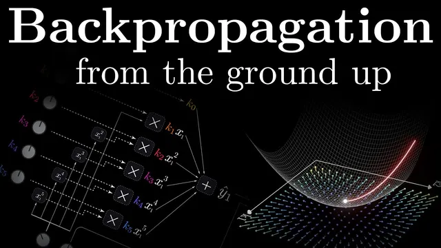
The explanation starts with an optimization problem that looks nothing like neural networks. Given data points (x, y), the task is to fit a curve y(x) by choosing parameters (in the example, polynomial coefficients k0 through k5). Because there are infinitely many possible curves, the discussion introduces an objective metric: a loss function. Using squared distance between predicted values and observed y values, the loss becomes a single number that depends on the parameters. Training then means finding the parameter setting that minimizes this loss.

A naive approach would try random perturbations: tweak one coefficient at a time, measure whether the loss improves, and repeat. That works in principle but wastes computation because it doesn’t use information about how the loss changes. The key upgrade is to know the direction in which each parameter should move. That direction comes from derivatives—specifically, the slope of the loss function with respect to each parameter. In one dimension, the derivative at a point tells how the loss changes for a tiny knob adjustment; at the minimum, the derivative becomes zero. In multiple dimensions, the same idea generalizes into partial derivatives and a gradient vector, which points toward steepest increase. To minimize loss, parameters move in the opposite direction of the gradient.

The central technical hurdle is how to compute these derivatives for complicated models. The solution relies on calculus rules, especially the chain rule, which describes how derivatives behave when functions are composed. By viewing a model as a sequence of simple differentiable operations—additions, multiplications, powers, nonlinear activations—derivatives can be propagated through the computation. This is where backpropagation earns its name: a forward pass computes the loss by running operations from inputs to output, while a backward pass runs the same computation graph in reverse to distribute gradients from the loss back to each parameter.

The transcript illustrates this with a computational graph. Each node represents a basic operation with known derivative behavior. When gradients flow backward, addition nodes pass gradients unchanged, multiplication nodes scale gradients by the other factor, and branching nodes sum gradients from multiple paths. Once gradients reach the parameter nodes, one training step updates each parameter by subtracting the gradient scaled by a learning rate. Repeating forward and backward passes yields the iterative training loop used across differentiable machine learning systems.

Finally, the discussion connects the method to neural networks: feed-forward networks can be decomposed into differentiable operations, so backpropagation can compute how each connection weight affects the loss. The result is an efficient optimization procedure that makes large-scale learning feasible. The next installment is framed around a comparison to biological learning, asking whether brains use an analogous mechanism like backpropagation or something fundamentally different.

Cornell Notes

Backpropagation is the mechanism that makes training differentiable models practical: it computes gradients of a loss function with respect to all parameters. Training then uses gradient descent, repeatedly updating parameters in the opposite direction of the gradient to reduce error. The method works by representing computations as a graph of simple differentiable operations and applying the chain rule. A forward pass calculates the loss, and a backward pass propagates derivatives from the loss back through the graph to each parameter. This gradient information turns “which way should each knob move?” into a systematic calculation, enabling scaling from toy problems (like polynomial curve fitting) to large neural networks.

Why introduce a loss function when fitting data with a curve?

Because there are infinitely many candidate functions, the process needs an objective measure of fit. In the example, the curve is a 5th-degree polynomial with coefficients k0 through k5. For each parameter setting, the model predicts y-values, compares them to observed data, and computes a single loss number—specifically using squared distances between predicted and actual y. Minimizing this loss turns curve fitting into an optimization problem over the parameters.

How does the “knob” picture lead to gradient descent?

With one adjustable parameter, the loss as a function of that parameter has a minimum where the derivative is zero. The derivative tells the local slope: if the derivative is negative, increasing the parameter decreases loss, so the update should move in the direction opposite the derivative. With multiple parameters, partial derivatives form a gradient vector; it points toward steepest increase. Gradient descent updates parameters by moving opposite the gradient, like rolling downhill toward a valley.

What does the chain rule contribute to backpropagation?

The chain rule explains how derivatives behave when one function feeds into another. If a model is built from composed operations (e.g., x → j(x) → f(j(x))), then the derivative of the overall output with respect to the original input depends on both derivatives: how j changes and how f changes with its input. Backpropagation applies this repeatedly across a computation graph so gradients can be computed for complex models from simple building blocks.

What exactly happens in the forward pass versus the backward pass?

The forward pass computes the loss by running operations from inputs to output (e.g., computing predicted values, then summing squared errors). The backward pass runs the same computation graph in reverse to compute gradients. Starting with the loss node (whose gradient is 1), each operation distributes the downstream gradient to its inputs using known derivative rules (addition passes gradients through, multiplication scales them, and branches sum gradients).

How do gradient updates use learning rate and why must gradients be recomputed?

After computing gradients, one training step updates each parameter by subtracting learning_rate × gradient (moving opposite the gradient). Because the parameter update changes the model and therefore changes the loss landscape, the old gradients no longer match the new configuration. The process repeats: forward pass to compute the new loss and backward pass to compute new gradients, then another update.

Review Questions

In the polynomial curve-fitting example, what are the parameters being optimized, and what is the loss function measuring?
How do partial derivatives and the gradient vector generalize the “slope tells you which way to move” idea from one knob to many knobs?
Why can backpropagation compute gradients efficiently without trying random perturbations of parameters?

Key Points

1
Modern machine learning training relies on minimizing a loss function by updating parameters using gradients computed via backpropagation.
2
Loss functions convert “how good is the prediction?” into a single numerical objective, often built from squared errors in the examples.
3
Derivatives tell how loss changes under tiny parameter changes; in multiple dimensions, partial derivatives combine into a gradient vector.
4
Gradient descent iteratively updates parameters by moving opposite the gradient, scaled by a learning rate.
5
Backpropagation computes gradients efficiently by applying the chain rule across a computation graph of differentiable operations.
6
A forward pass computes the loss, while a backward pass propagates gradients from the loss back to each parameter using operation-specific rules.
7
As long as a model can be decomposed into differentiable building blocks, the same forward/backward gradient loop can train it.

Highlights

Backpropagation turns the “which way should each parameter move?” question into a chain-rule-based gradient calculation.

A forward pass computes the loss; a backward pass distributes derivatives through the computation graph until parameter gradients are known.

In gradient descent, the gradient vector points toward steepest increase, so minimizing loss means stepping in the opposite direction.

Random perturbations can work but waste computation; derivatives provide local direction information that makes optimization efficient.

The method scales because neural networks can be expressed as compositions of differentiable operations (adds, multiplies, nonlinearities).

Topics

Mentioned

David Rumelhart
Geoffrey Hinton
Ronald Williams
Seppo Linnema